Even a Rough Model Can Make Rare Blackouts Cheaper to Measure
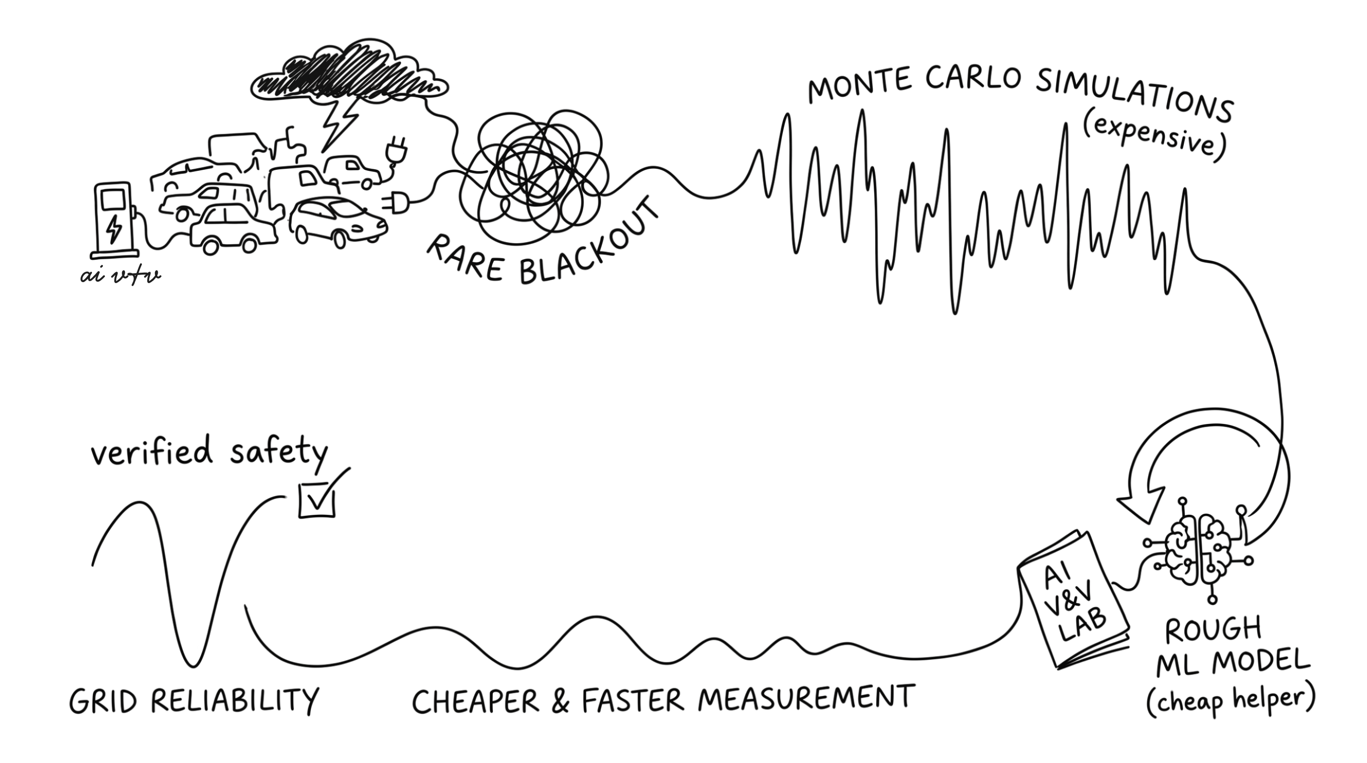
On a normal day, the power line that feeds a public charging station has plenty of spare capacity. The trouble comes on the rare day when several things go wrong at once. A heat wave pushes every air conditioner in the area to full power, the utility’s forecast for the day comes in too low, a storm shifts extra load onto the line, and a crowd of drivers arrives to charge at the same time.
If the load climbs past the line’s limit, protective equipment switches the line off. The charging station goes dark, along with every home and shop on the same line. The load that was on it then moves to neighboring lines, which can overheat in turn. Large blackouts have started this way, including the August 2003 blackout that cut power to about 50 million people in the United States and Canada.
So before a utility approves a new charging station, it wants to know how often this could happen. A common standard in power planning allows no more than one blackout day in ten years. That is a daily chance of about 1 in 3,650.
Checking a number that small is expensive. Utilities answer the question with computer simulations of the grid, and each simulated day takes real computing time. The standard approach, called Monte Carlo simulation, runs the model over many randomly drawn days and counts how often the line fails. To pin down the answer within 10 percent, it needs to see about 400 failures. At a rate of 1 in 3,650, that means roughly 1.5 million simulated days. For stricter targets, such as 1 in a million, it means about 400 million.
In a new paper by Sulyman Iyanda and Mansur Arief, submitted to the 2026 IEEE International Conference on Smart Grid and Smart Cities (ICSGSC), we show that a fairly simple machine learning model can cut that cost by more than half. The model only needs to be a little better than a coin flip at spotting bad days. The code is public on GitHub.
A cheap helper that corrects for luck
The idea behind the method is an old one in statistics, known as a control variate. Suppose you want the average of something that is expensive to measure, and you also have something cheap that tends to move with it. If you know the true average of the cheap thing, you can use it to see how lucky or unlucky your sample was, and correct for it.
Here is how that works for blackouts. Say a batch of simulated days happens to include more heat waves than a typical year would. The blackout count from that batch will come out too high. The cheap signal will also come out too high, and since we know what its average should be, we can measure the excess and adjust the blackout estimate down. When the batch has fewer heat waves than usual, the adjustment goes the other way. On average the adjustment is zero, so it never pushes the answer in one direction.
In earlier work on charging stations in Surabaya, Indonesia, our group used this trick with a cheap signal built from a bell-curve (Gaussian) model of electricity demand. The new paper replaces that signal with a machine learning classifier. The classifier looks at information a utility already has before any simulation runs, such as the temperature, the day-ahead load forecast, and whether a storm is expected. From these it guesses whether the day will end in an overload.
The classifier is trained once, on a modest number of simulator runs. Its average alarm rate can then be worked out from years of past weather records, which costs almost nothing because no grid simulation is needed for that step.
Why a mediocre model is good enough
The paper’s first result is a simple formula for how much the classifier helps. The answer depends on two numbers that anyone who has worked with classifiers will know. Recall is the share of real overload days that the model flags. Precision is the share of the model’s alarms that turn out to be real overload days.
When overloads are very rare, the noise left in the estimate shrinks to about (1 − recall × precision) of what plain Monte Carlo would leave. A model that catches half the bad days, and is right half the time it raises an alarm, removes about a quarter of the noise. That is like getting a third more simulations for free.
Any model that does better than chance helps at least a little. It does not need high accuracy in the usual sense, and its scores do not need to be well-calibrated probabilities.
There is one catch, and it is an important one. Recall is easy to get, since a model that sounds the alarm every day will catch every overload. Precision is much harder. If the model’s false alarms stay at a fixed level while real overloads become rarer, its precision falls toward zero and its benefit disappears with it. A forecasting model judged by everyday accuracy can look fine and still be of little use here. For this job, the model’s alarms have to stay meaningful on the rarest days.
Where the bell curve falls short
The same reasoning explains why the earlier bell-curve shortcut stops working. Bell-curve models are convenient, and two bell-curve quantities that move together on ordinary days look like a good match. Statisticians have known since the 1960s that such pairs drift apart at the extremes. On the most unusual days, which are the only days that matter for blackouts, knowing one tells you little about the other.
The paper proves that a bell-curve signal loses all of its value as the target becomes rarer, however closely it follows demand on normal days. In our tests, a realistic version removed less than 0.2 percent of the noise. Even an unrealistically good one, which tracked demand with a correlation of 0.98, kept losing ground as the target got stricter.
A second result puts an upper limit on what any model can do. How much a classifier can help depends on how much the input data says about the bad days. If overloads are driven by things the utility can see, such as heat, forecast errors and storms, a good model can do well. If they are mostly driven by random factors that nobody measures, no model can help much. In our simulator, cutting the hidden randomness in half raised this ceiling from 64 percent to 79 percent of the noise. Doubling it lowered the ceiling to 38 percent. For a utility, better data about each day is worth more than a fancier model.
Training on the bad days
Training such a model has a practical problem. If it learns from ordinary days, it almost never sees an overload, so it learns little about them. Our tests showed this clearly. A boosted-tree model, a common and strong type of classifier, trained on 10,000 ordinary simulated days removed 34 percent of the noise at a target of 1 in 1,000. At 1 in 10,000 it removed 5 percent, and below that it removed nothing.
The fix is to train the model mostly on hot days with high forecasts, where overloads actually happen. The paper shows that this is allowed. As long as the training runs are kept separate from the runs used for the estimate, the estimate stays unbiased no matter which days were used for training.
There is a second benefit. The simulator reports the peak load on the line as a number, so one set of training runs can be relabeled for any capacity limit. A utility can train the model once and reuse it when line ratings, reliability targets or station plans change.
What the tests showed
We built a simplified simulator of a power line with three inputs a utility would know in advance (temperature, forecast error and a storm flag), plus hidden randomness that it would not know. We set the line’s limit so that the true overload rate was exactly 1 in 1,000, 1 in 10,000, 1 in 100,000 or 1 in a million. Because we designed the simulator ourselves, we could compute the right answer in every case and check each method against it. The methods themselves never had access to that answer.
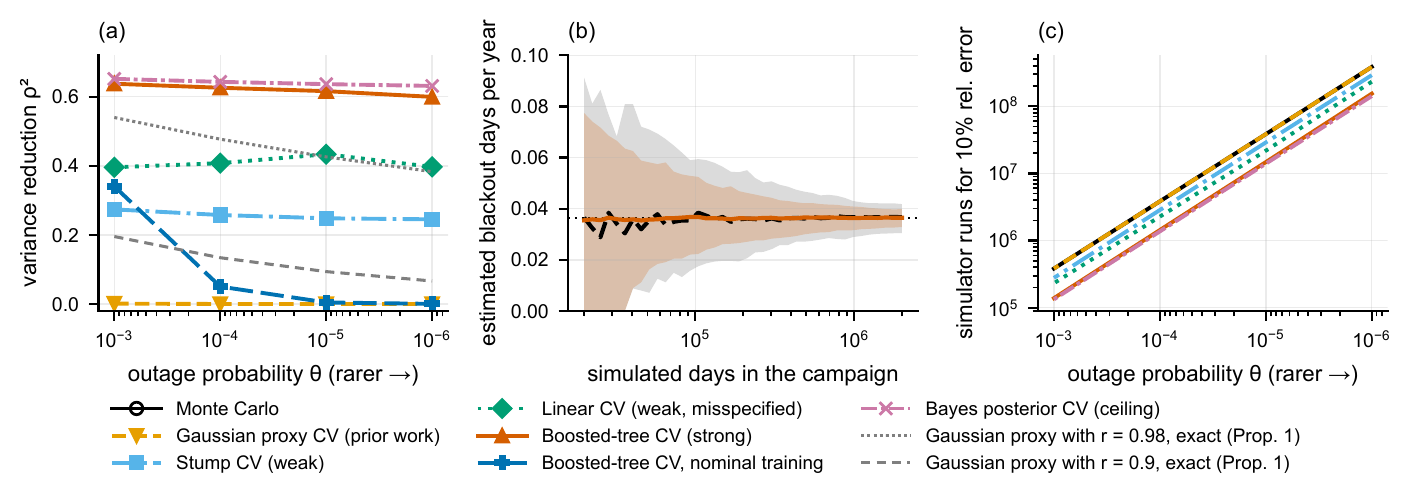 Figure 1. (a) Share of the noise each method removes as overloads become rarer. (b) How the estimate settles as more days are simulated, for plain Monte Carlo (dashed) and the boosted-tree helper (solid), with shaded bands covering 95 percent of 400 repeated runs. (c) Number of simulated days needed to get within 10 percent of the true answer.
Figure 1 shows how each method held up as overloads became rarer. A one-rule model, which only checks whether the temperature is above a threshold, removed about a quarter of the noise at every level. That saves about 1.3 times the simulations. A simple straight-line model removed about 40 percent, a saving of 1.7 times. The boosted-tree model, trained on bad days, removed 60 to 64 percent. It cut the number of simulations by a factor of 2.5 to 2.8 and came within 5 percent of the best any model could do with these inputs. The bell-curve signal removed almost nothing.
We repeated each method hundreds of times. The errors matched what the formulas predicted, and the 95 percent confidence ranges contained the true value 92 to 98 percent of the time. At the 1-in-a-million level, getting within 10 percent took about 380 million simulated days with plain Monte Carlo. With the boosted-tree helper it took about 150 million, plus a one-time cost of about 12,000 runs to train the model.
The tests also turned up one warning. When a batch contained only two or three overloads, the helper sometimes made the estimate worse, because the adjustment was being tuned on too few bad days. From about 20 overloads onward, it behaved as expected.
A blackout map of Surabaya
To see what this means for a real planning decision, we went back to the Surabaya network from our earlier study. It has 11 feeders, the local power lines that carry electricity to neighborhoods, serving 31 districts. We placed a charging station on each feeder and asked how much extra capacity each one would need, through an upgrade or a cap on charging, to meet the one-day-in-ten-years standard. That standard works out to 0.1 expected blackout days per year. Our simulator matches each feeder’s reported reliability today and differs from the bell-curve model only on extreme days.
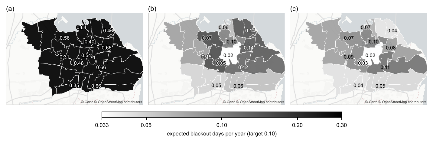 Figure 2. Expected blackout days per year in each Surabaya district after a charging station is added and capacity is planned using (a) the bell-curve model, (b) plain Monte Carlo with 10,000 simulated days per feeder, and (c) the learned helper on the same days with a 95 percent safety margin. The target is 0.10 days per year.
With the bell-curve model, every feeder came up short. The true blackout rate landed between 0.31 and 0.66 days per year, three to seven times the standard, for a city total of 5.7 blackout days per year across all feeders.
With plain Monte Carlo on 10,000 simulated days per feeder, sized to the best guess, 46 percent of the feeders still missed the target. The planner also had no way of telling which ones. With the learned helper on the same 10,000 days, plus a 95 percent safety margin, only 15 percent missed it, and none missed by more than double. The city total fell from 1.17 to 0.77 blackout days per year. The share of residents served by a feeder that missed the standard fell from 46 percent to 15 percent.
Much of that gain comes from the safety margin itself, since plain Monte Carlo with the same margin reaches 0.78 days. The learned helper then cuts the share of feeders that miss the target from 24 percent to 15 percent.
The cost side shows up on the largest feeder, Embong Wungu. It needs an upgrade of about 29 percent of its base load, while the bell-curve model asks for only 18 percent. When both methods use the safety margin, plain Monte Carlo builds in more spare capacity than the feeder needs. With 20,000 simulated days, it overbuilds by 1,420 load units on average (the data are scaled for privacy), compared with 816 units for the learned helper. Put simply, the helper gives the same quality of decision as a Monte Carlo study two to three times larger.
What this means for utilities
A few practical lessons come out of the results. The first is to invest in data before models. The ceiling on any model is set by what the utility records about each day, such as past line loads, maintenance schedules and the load forecasts it already produces. A more complex model trained on the same inputs cannot raise that ceiling.
The second is to spend the training budget on the dangerous days. A model trained on hot, high-demand days keeps its value at every reliability target, and it can be reused when plans change. A model trained on typical days is close to worthless for rare events.
The third is that the helper only needs the inputs for each day, so it can be run over a decade of weather records at almost no cost. The paper gives a formula for how many such archive days are worth one grid simulation.
Put together, the recipe is short. Train once on a sample focused on the dangerous days. Run the model over the weather archive. Size the reserve using an upper safety margin, and wait until the simulations contain about 20 overloads before making the call.
What comes next
This work is part of our lab’s research on measuring rare failures, which we described in Why Your AI Needs Scalable Verification and Validation. Much of that research uses a different method, called importance sampling, which deliberately simulates more of the dangerous cases and then corrects the count. Importance sampling can be very efficient, but someone has to show that it has not missed any of the ways a system can fail. The learned helper in this paper keeps the normal sampling, so it is safe to use even when the model behind it is imperfect. The two methods fit well together.
The study has limits we plan to address. The simulator is synthetic, which let us check every answer exactly, but its behavior on extreme days is assumed. Next we want to drive it with real weather and outage records. We also treated each feeder on its own, even though a citywide storm affects many feeders at once. Finally, we picked the “dangerous days” for training by hand. An adaptive approach that combines this learned helper with learned importance sampling is where we plan to take the work next.
Readers who want to reproduce the figures, or test their own model on the simulator, can start from the code repository. As with our deepbullwhip release, we hope others will add their own methods to the comparison.
References
- S. Iyanda and M. Arief, “Learned Control Variates for Rare Grid-Outage Estimation at Electric Vehicle Charging Stations,” submitted to the IEEE International Conference on Smart Grid and Smart Cities (ICSGSC 2026), Guangzhou, December 2026. Code at github.com/ai-vnv/learned-control-variates-rare-outages.
- Y. P. Akhra, I. Vanany and M. M. Arief, “A Robust Electric Vehicle Charging Station Optimization under Rare Event Disruptions,” arXiv:2307.05470v2. The Surabaya case study and the bell-curve helper this paper builds on.
- R. Billinton and R. N. Allan, Reliability Evaluation of Power Systems, 2nd ed., Plenum Press, New York, 1996. Source of the one-day-in-ten-years standard.
- U.S.-Canada Power System Outage Task Force, Final Report on the August 14, 2003 Blackout in the United States and Canada, 2004. Available from the U.S. Department of Energy.
- I. Dobson, B. A. Carreras, V. E. Lynch and D. E. Newman, “Complex systems analysis of series of blackouts: Cascading failure, critical points, and self-organization,” Chaos 17, 026103, 2007. doi:10.1063/1.2737822. How local overloads grow into large blackouts.
- M. Sibuya, “Bivariate extreme statistics,” Annals of the Institute of Statistical Mathematics 11, 195–210, 1960. doi:10.1007/BF01682329. Why bell-curve pairs drift apart at the extremes.
- R. E. Schapire, “The strength of weak learnability,” Machine Learning 5, 197–227, 1990. doi:10.1007/BF00116037. The idea of a model that is only slightly better than chance.
- M. Arief et al., “Deep probabilistic accelerated evaluation: A robust certifiable rare-event simulation methodology for black-box safety-critical systems,” AISTATS 2021. arXiv:2006.15722. Our earlier work on learned importance sampling.