Catalyzing Supply Chain Research with Open Benchmarks and deepbullwhip

In October 2025, the Dutch government seized Nexperia and split the company into Dutch and Chinese entities. China retaliated with export controls, wafer shipments halted, and discrete-component lead times stretched by six to eight weeks beyond their prior baselines. At almost the same time, memory prices for popular DDR4 and DDR5 configurations quadrupled between September and November 2025, with Deloitte projecting further 50 percent increases through the first half of 2026 and one semiconductor distributor reporting 1,000 percent inflation on specific parts. Apple, Tesla, and a suite of other manufacturers have warned shareholders that DRAM constraints will throttle 2026 production. Industry insiders have taken to calling it “RAMageddon.”
These events sit on top of a much older problem. The bullwhip effect, the tendency for order variability to amplify as information moves upstream through a supply chain, has been studied since Jay Forrester’s Industrial Dynamics in 1961. Lee, Padmanabhan, and Whang formalized its four root causes in 1997. Chen and colleagues derived tight lower bounds on the bullwhip ratio under Order-Up-To policies in 2000. Decades of analytical progress have mapped the mechanics. And yet the 2020 to 2022 chip shortage, the 2025 to 2026 memory crisis, and the Nexperia shock all show the same signature of panic ordering, capacity double-booking, and price correction that theory has been describing all along.
Our lab thinks a piece of the reason is computational. The tools that researchers use to study the bullwhip effect have not kept pace with the theory, and more importantly, they have not kept pace with the benchmarking standards that other fields now take for granted. Today we are releasing deepbullwhip, an open-source Python package that tries to close that gap. The accompanying arXiv preprint describes the design, the validation against analytical bounds, and five sets of experiments on a four-echelon semiconductor supply chain.
Why another simulator
The existing landscape of bullwhip tools has clear gaps. AnyLogic and Arena are powerful, but proprietary and license-restricted. The Beer Distribution Game that John Sterman has used to teach generations of managers is pedagogically brilliant but fixed in its four-echelon structure and deterministic demand. General-purpose open-source libraries like supplychainpy and frePPLe solve adjacent problems (demand classification, production scheduling) rather than multi-echelon bullwhip propagation with asymmetric newsvendor costs. The predominant mode in the research literature is ad hoc simulation, where custom scripts are written per paper in MATLAB, Python, or R, tightly coupled to specific assumptions, and rarely reusable.
A related and arguably more consequential shortcoming is the absence of a standardized benchmarking protocol. Studies select metrics inconsistently, test against different demand processes, and compare against different baseline policies, which makes cross-study comparison unreliable. The forecasting community solved an analogous problem through the M-competitions that established shared datasets and evaluation protocols, and MMDetection and Detectron2 play similar roles for computer vision. No equivalent infrastructure exists for bullwhip research.
What deepbullwhip is
deepbullwhip combines two things. The first is a modular simulation engine where demand generators, ordering policies, cost functions, and forecasters are all substitutable through abstract base classes. A vectorized Monte Carlo engine processes over 20 million simulation cells in under 7 seconds on a single CPU core. The second is a registry-based benchmarking framework that ships a curated catalog of ordering policies, forecasters, six bullwhip and cost metrics, and demand datasets including WSTS semiconductor billings and M5 Walmart retail data.
Getting started is one line:
pip install deepbullwhip
A minimal simulation is five lines:
from deepbullwhip import SemiconductorDemandGenerator, SerialSupplyChain
import numpy as np

gen = SemiconductorDemandGenerator()
d = gen.generate(T=156, seed=42)
chain = SerialSupplyChain()
result = chain.simulate(d, np.full_like(d, d.mean()),
                        np.full_like(d, d.std()))
The full API documentation lives at ai-vnv.github.io/deepbullwhip. The package is MIT-licensed, which matters for industry partners who need to link against or modify the code without legal friction.
What the experiments revealed
We ran five sets of experiments on a four-echelon semiconductor chain configured with the lead times reported in Mönch, Fowler, and Mason’s text: the distributor at 2 weeks, the OSAT assembly and test tier at 4 weeks, the foundry at 12 weeks, and the wafer supplier at 8 weeks. Four findings stood out.
The first was how aggressively amplification compounds. Under a standard Order-Up-To policy, the Monte Carlo mean cumulative bullwhip ratio across 1,000 paths reached 427. Meaning a dollar of demand variance at the distributor turned into 427 dollars of variance at the wafer supplier. Single-path simulation with a structural shock at week 104 produced a cumulative ratio of 838, with E4 order spikes exceeding 1,000 units against a baseline demand of roughly 12 units. The multiplicative cascade across echelons is the culprit, and it dwarfs the single-tier bounds that most analytical papers stop at.
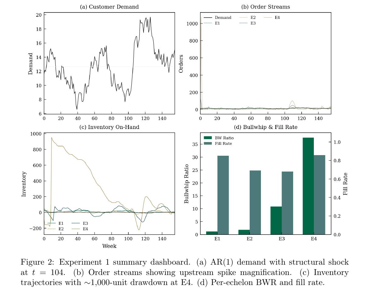 Figure 2 from the paper. Panel (a) shows a single realization of AR(1) customer demand with a structural shock at week 104. Panel (b) shows how that demand propagates into order streams across echelons, with the E4 supplier’s opening order exceeding 1,000 units against a demand baseline of roughly 12. Panel (c) shows the inventory trajectory, including a drawdown of nearly 1,000 units at E4 that represents substantial working capital exposure. Panel (d) summarizes the per-echelon bullwhip ratio climbing from 1.1 at the distributor to 37.6 at the wafer supplier. The cumulative ratio on this path is 838.
The second was a stochastic filtering phenomenon that, as far as we can tell, has not been documented before. Running 1,000 Monte Carlo paths and computing the coefficient of variation of BWR at each echelon produced a striking asymmetry. The distributor tier showed CV of 0.21, with BWR varying substantially across demand realizations. The foundry tier showed CV of 0.01, with BWR almost deterministic regardless of what demand looked like. We formalized this through a delta-method argument (Proposition 1 in the paper) that shows why the ratio becomes near-deterministic at upstream tiers where the demand cascade induces high correlation between successive order variances. The prediction matched the empirical CV to four decimal places at the foundry tier, and the cumulative-BWR extension (Corollary 1) predicted CV(BWR_cum) within 1.8 percent of the empirical value across 5,000 paths. The operational implication is that upstream capacity planners can lean on deterministic scenario analysis, while distributor-tier planners need stochastic evaluation to characterize their path-dependent risk.
The third was the BWR–NSAmp tradeoff. The Proportional Order-Up-To (POUT) policy with smoothing parameter α = 0.3 reduced cumulative BWR by 96 percent, from 427 to 16.3. That sounds like an unambiguous win until you look at the other metrics. Fill rate at the distributor collapsed to near zero, total cost at that tier rose from 293 to 2,377, and the Smoothing OUT variant preserved fill rates but quadrupled inventory variance at the wafer tier. Sweeping α from 1.0 down to 0.1 traced a Pareto frontier with non-monotonic inventory response, and varying the backorder-to-holding cost ratio from 2 to 20 reversed the policy rankings. No single metric captures policy quality, which is exactly why multi-metric benchmarking matters.
The fourth finding is the one that should worry practitioners. We replayed 60 months of WSTS semiconductor billings through the same chain and compared cumulative BWR against the synthetic AR(1) demand process that most analytical papers use. The synthetic process produced cumulative BWR of 429. The real WSTS data produced 66,076. A gap of roughly 155 times.
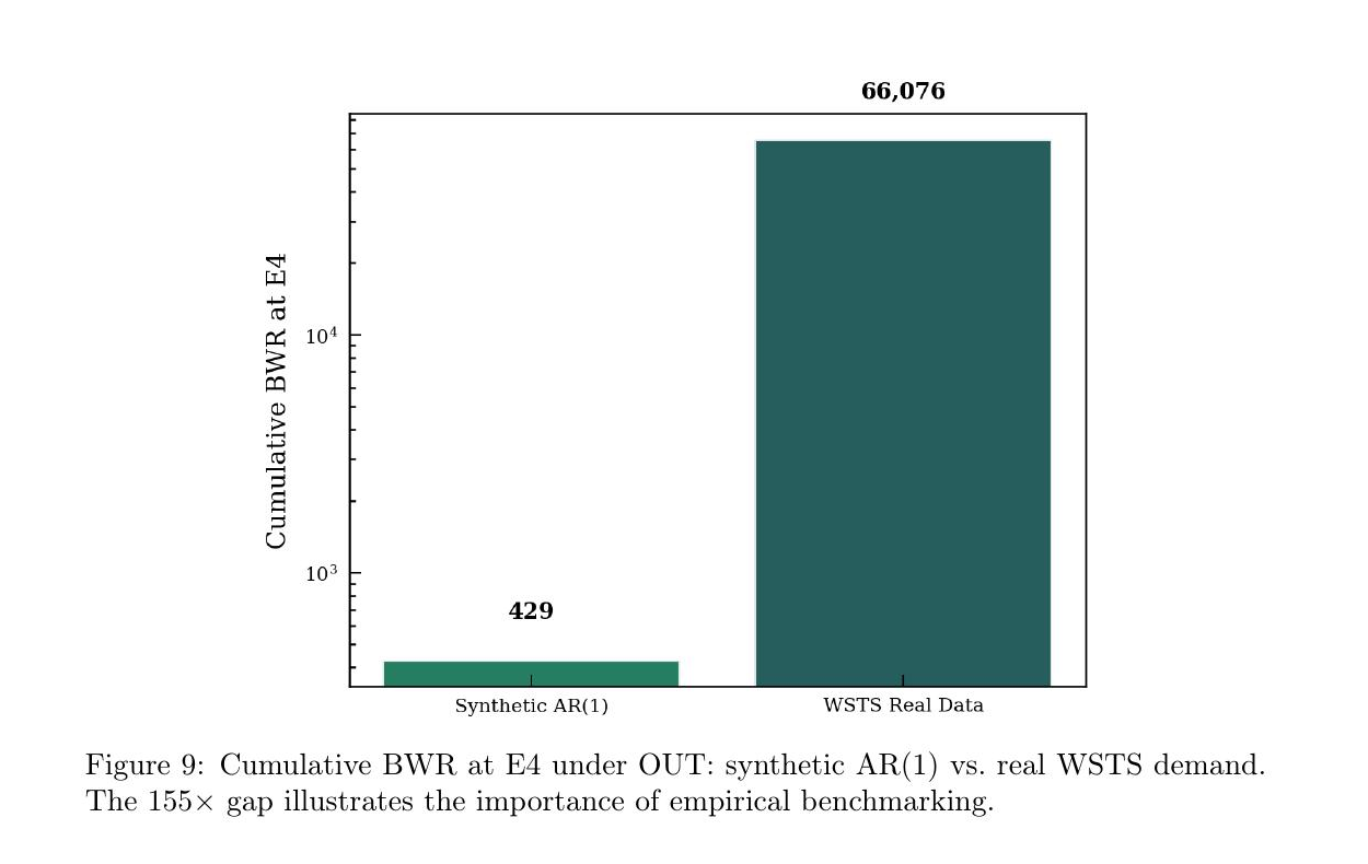 Figure 9 from the paper. Cumulative bullwhip ratio at E4 under the Order-Up-To policy, comparing synthetic AR(1) demand against a replay of 60 months of World Semiconductor Trade Statistics billings. The 155-fold gap is shown on a log scale, which itself understates how stark the absolute difference is.
The WSTS series has regime-switching behavior around the 2019 trade-war downturn, the 2020 to 2021 pandemic surge, and structural breaks that a stationary AR(1) model cannot capture. Inventory planning tools validated on synthetic demand can underestimate operational risk by two orders of magnitude.
Why this matters for today’s crises
The timing of this release is not incidental. The semiconductor industry is living through the third major supply-chain shock of the decade. CoWoS advanced packaging capacity is fully booked through 2027. Equipment lead times for lithography and etch tools run 18 to 24 months. Chinese export restrictions on gallium, germanium, and tungsten are tightening. The decisions being made right now, about how aggressively to order, how much safety stock to carry, how much smoothing to apply, will shape costs and service levels for the next several years.
The 155-fold synthetic-versus-real gap is a cautionary message for anyone using simulation tools calibrated only on textbook demand processes. The stochastic filtering result says that upstream tiers, precisely the foundry and wafer suppliers where most of the cost is incurred, can be analyzed deterministically, which changes how capacity planning software should be architected. The BWR–NSAmp tradeoff says that adopting a smoothing policy without testing it against multiple metrics and cost structures is a good way to trade a variance problem for a fill-rate problem.
None of this replaces analytical theory or operator judgment. It does give both a shared substrate to argue over.
How this fits into the lab’s research
Our lab’s mission is to raise the trustworthiness of AI systems through verification and validation, and supply chain applications are one of the three pillars we focus on alongside neural network verification and autonomous systems. The accuracy–robustness tradeoff in ML-driven inventory decisions that Ban and Rudin documented in 2019 is, at its heart, a verification question. A forecaster that improves point accuracy by 20 percent but worsens multi-echelon cost is not a “better” system in any operationally meaningful sense. Evaluating such claims requires infrastructure that our lab thinks should be open, reproducible, and shared.
deepbullwhip is part of a broader effort to push supply chain research toward higher technology readiness levels by meeting three conditions the field has historically lacked. Benchmarks that let methods be compared on equal footing. Real-data replay that stress-tests conclusions drawn from synthetic processes. And an extension mechanism (the decorator-based registry) that lets a researcher contribute a new policy, forecaster, or metric with a single decorated class and have it evaluated against every baseline in the catalog. This is the pattern that worked for computer vision benchmarks and robustness testing in deep learning, and we think it can work for operations research too.
We have already integrated DeepAR as a first deep-learning baseline, and the registry is designed to accept deep reinforcement learning inventory policies and end-to-end newsvendor networks without code modification. Convergent and divergent chain topologies, capacity constraints, and multi-product demand with substitution are on the near-term roadmap.
Try it, break it, extend it
The package is live on PyPI and GitHub, with full API documentation and reproducible Jupyter notebooks for every experiment in the paper. We genuinely want researchers and practitioners to kick the tires. Register a policy that we have not thought of. Replay a proprietary demand series we cannot access. Tell us where the simulator gives wrong answers, where the abstractions break, and where the benchmarking interface is missing something obvious. Issues and pull requests are welcome, and the leaderboard is intended as a long-running community resource rather than a one-time release.
The bullwhip effect is 65 years old as a concept and still costing the global economy hundreds of billions of dollars in every cycle. Moving that number requires closing the loop between analytical theory and operational reality, and that loop closes faster when the infrastructure is shared.